Understanding the Markov Chain Attribution Model: A Deep Dive into Customer Journey Analysis

If you’ve ever tried to answer “Which channels actually move the needle across our full customer journey?”, you’ve probably run into the limits of last click, linear, or even platform-specific “data-driven” models. The Markov chain attribution (MCA) model is a practical, sequence-aware approach that turns raw journeys into transition probabilities and then estimates each channel’s incremental contribution via the removal effect. In plain English: it quantifies what would happen to your conversion rate if a given channel disappeared from the path mix.

In this ultimate guide, I’ll cover the concept, the math intuition (not heavy), the end-to-end implementation workflow, robustness checks, how to operationalize results, and where MCA fits alongside Shapley value models, GA4’s Data-Driven Attribution, MMM, and experiments. I’ll keep the lens on e-commerce (Shopify/DTC), but the methods generalize well.

1) Why Markov chain attribution for e-commerce?

• It respects sequence. Prospecting social followed by branded search is not the same as the reverse order; MCA captures that difference through transition probabilities.
• It’s interpretable. You can inspect the transition matrix and see which steps most often precede conversion.
• It’s actionable. The removal effect translates into budget reallocation logic: if removing Paid Social drops overall conversion probability notably, that channel is contributing incrementally to the system.
• It plays well with privacy-era realities. You can model with your own first-party paths and complement gaps with privacy-safe aggregates from clean rooms.

That said, MCA is not a causal model by default. Treat removal effect as a structural contribution signal, then triangulate with incrementality tests before making big budget moves.

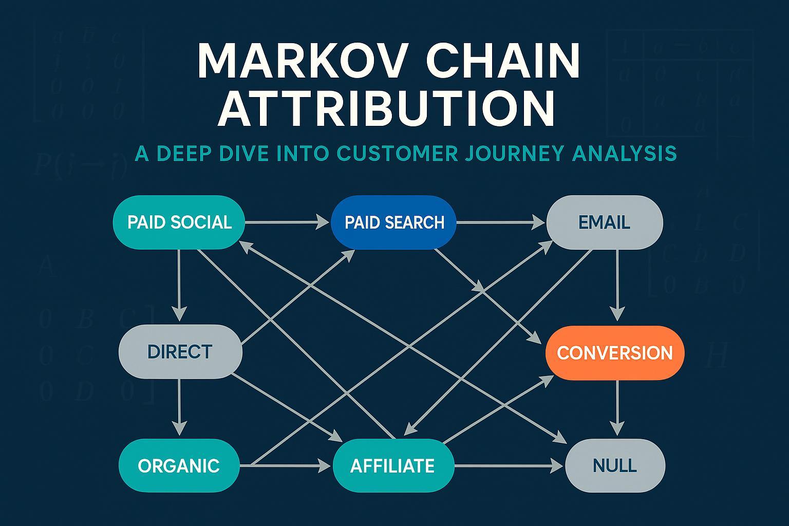
2) The core intuition: states, transitions, and absorbing endpoints

Mark the customer journey as a chain of states (touchpoints) connected by probabilities. Two special absorbing states end the path: Conversion and Null (no conversion within the window). Once a path reaches either, it stops.

• Transient states: Paid Social, Paid Search (Brand/Non-Brand), Organic Search, Email/SMS, Display, Affiliate, Direct, Referral, etc.
• Absorbing states: Conversion, Null
• Special start state: Start (or “Landing” if you prefer), which begins every path.

According to Google’s documentation (current as of 2025), the Markov analysis implemented in Ads Data Hub operates on sequences of touchpoints and computes channel credit by simulating “what if this channel didn’t exist,” commonly referred to as the removal effect. See the official description in the Google Developers — Ads Data Hub Markov chain analysis.

3) Removal effect, demystified (with a toy example)

Think of a simplified path universe:

• Start → Paid Social → Branded Search → Conversion
• Start → Organic → Conversion
• Start → Paid Social → Direct → Null

From these observed paths, you build a transition matrix: for each state, what fraction of the time does the next step go to each possible state?

• Baseline conversion probability: simulate many journeys from Start using those probabilities until they hit Conversion or Null. You can compute this analytically from the matrix as well.
• Removal effect for a channel X: Remove state X, reconnect its inbound transitions to its outbound transitions, recompute baseline conversion probability, and measure the drop. Larger drops imply greater incremental contribution.

Important nuance: A high removal effect means the channel helps the path ecosystem reach conversion more often, given the observed sequences. It is still not a randomized causal estimate; always validate with experiments when stakes are high.

4) Data and path preparation (the 80% that decides success)

You can’t fix attribution with modeling if your path data is inconsistent. Invest here.

• Identity and stitching

  • Prefer consented first-party IDs (hashed email/login), with device/session joins where allowed.
  • De-duplicate events and order strictly by timestamp.
  • Decide how to collapse repeated exposures (e.g., multiple paid social impressions in 60 minutes) to reduce loops.

• Channel taxonomy

  • Separate Paid Search Brand vs Non-Brand.
  • Split Paid Social Prospecting vs Retargeting.
  • Disambiguate Direct vs true last-touch captures from affiliates/coupon sites.
  • Aggregate micro-campaigns to channel families to avoid sparsity.

• Lookback windows and inclusion rules

  • Define the conversion window per business cycle (e.g., 7, 30, or 90 days). For GA4 properties, lookback settings live in Admin → Attribution Settings; details are outlined in the Google Analytics Help — Attribution settings (documentation current as of 2025).

• Path construction

  • Add Start at the beginning, Conversion/Null at the end.
  • Optionally segment models by cohort (new vs returning) or funnel (prospecting vs lifecycle).

• QA checklist

  • What share of paths are single-touch? If very high, ensure tracking completeness.
  • Do any states have extremely low support? Consider aggregating.
  • Are branded search touches overrepresented right before Conversion? Consider segmenting or downweighting via time decay.

5) Step-by-step implementation workflow

Here’s a vendor-agnostic blueprint you can execute in SQL + Python/R.

5.1 Extract transition counts

• From each ordered path, emit adjacent pairs including Start → first touch and last touch → absorbing state (Conversion or Null).
• Count transitions by from_state, to_state.

Example SQL sketch (BigQuery syntax-like):

-- paths(table): user_id, ts, channel, is_conversion
-- Assume paths are pre-ordered and cleaned.
WITH steps AS (
  SELECT user_id,
         ARRAY_CONCAT([STRUCT('Start' AS channel)], ARRAY_AGG(channel), [STRUCT(IF(MAX(is_conversion)=1,'Conversion','Null') AS channel)]) AS seq
  FROM paths
  GROUP BY user_id
), transitions AS (
  SELECT from_state, to_state, COUNT(*) AS cnt
  FROM (
    SELECT s.user_id,
           seq[offset(i)] AS from_state,
           seq[offset(i+1)] AS to_state
    FROM steps s, UNNEST(GENERATE_ARRAY(0, ARRAY_LENGTH(seq)-2)) AS i
  )
  GROUP BY from_state, to_state
)
SELECT * FROM transitions;

5.2 Normalize to probabilities and smooth

• For each from_state, row-normalize counts to probabilities.
• Apply additive smoothing (e.g., Laplace/Dirichlet α≈0.1–1.0) to avoid zero-probability edges that can destabilize simulations.

5.3 Choose model order and consider time decay

• Start with first-order (next step depends only on current). It’s typically more stable and data-efficient.
• If evidence suggests strong order dependence, use a back-off: second-order where counts are sufficient, otherwise fall back to first-order. Many practitioners stop here to avoid sparsity explosions.
• Optionally apply time decay before counting transitions so recent touches weigh more.

5.4 Compute baseline conversion probability

• Represent the chain as matrices: transient-to-transient (Q) and transient-to-absorbing (R). The probability of eventual conversion from Start can be derived via the fundamental matrix (I − Q)^{-1} R, or approximated via Monte Carlo simulations if that’s more practical in your stack.

5.5 Removal effect and credit allocation

• For each channel state C:
  1. Remove C (and its edges), reconnecting inbound → outbound transitions in proportion to C’s outbound probabilities.
  2. Recompute overall conversion probability from Start.
  3. Removal effect = baseline − new probability.
• Normalize removal effects across channels and multiply by total conversions (or revenue) to generate fractional credit.

An official description of this process and privacy-aware execution appears in the Google Developers — Ads Data Hub Markov chain analysis (Google documentation, current as of 2025).

5.6 Practical implementation options

• R/Python package: The open-source ChannelAttribution (R/Python) library provides k-order Markov and removal effect out of the box.
• Warehouse-first: Prepare transitions in BigQuery/Snowflake, export a compact matrix to Python/R for the removal-effect runs.
• Cost hygiene: If you’re on BigQuery, control costs with partitioned and clustered tables and pre-aggregations. Adswerve’s practitioner notes cover useful tactics in their GA4 BigQuery tips for attribution (industry article, 2024–2025).

6) Tools and data readiness (privacy-first pipeline)

You’ll need trustworthy first-party event streams and a way to integrate walled-garden exposure data safely.

• Server-side collection and identity:

  • Consider a server-side tracking pipeline that captures web events, honors consent, and enriches with first-party IDs. A platform like Attribuly supports server-side collection, identity resolution, and data activation across Shopify and major ad channels. Disclosure: Attribuly is our product.
  • For how multi-touch windows are handled in practice at our brand, see this brief note in the Attribuly FAQ on multi-touch and attribution windows.

• Clean rooms and platform data:

  • Use environments like Google Ads Data Hub (ADH) to analyze Google ecosystem exposures with privacy thresholds in place. Google’s docs explain user-provided data matching and outputs at an aggregated level in the Ads Data Hub user-provided data matching guide (Google Developers, current as of 2025).

• Warehouse and modeling:

  • Land all sources into BigQuery/Snowflake, normalize channels, and run the Markov model with open-source libraries.

Balance note: You can build an excellent MCA program with GA4 export to BigQuery + open-source modeling, or with ADH analyses where applicable. Choose based on your data governance and scale.

7) Robustness and validation: separating signals from noise

MCA can overreact to sparse or biased paths unless you harden it.

• Sparsity mitigation

  • Aggregate micro-states to channel families (e.g., all prospecting social campaigns → Paid Social Prospecting).
  • Apply additive smoothing on transitions to prevent zero-probability bottlenecks.
  • Set minimum support thresholds (e.g., exclude states with <N paths), and consider separate models for new vs returning users.

• Bias controls

  • Brand search proximity: Branded Paid Search often appears right before conversion; segment brand vs non-brand or new vs returning to avoid over-crediting.
  • Retargeting loops: Collapse repeated impressions within time buckets or apply time decay.
  • Opportunistic affiliates/coupon: Distinguish assist partners from last-second coupon captures.

• Statistical validation

  • Bootstrapping: Resample paths to generate confidence intervals around removal effects.
  • Holdouts and stability: Train on period A, evaluate on period B; check that channel rankings are reasonably stable.
  • Sensitivity analysis: Compare first-order vs limited second-order; vary smoothing constants; test alternative channel groupings.
  • Triangulation: Compare Markov results with Shapley allocations on the same data, inspect GA4 DDA trends, and, crucially, run geo/A–B experiments to confirm major reallocations. A 2025 technology survey from Statsig discusses the trade-offs across models in their digital marketing attribution models overview.

8) Where Markov fits vs Shapley, GA4 DDA, and MMM/Incrementality

• Markov (removal effect)

  • Strengths: Sequence-aware, intuitive via transition probabilities, computationally practical on realistic channel sets, good for “how do journeys behave?”
  • Limitations: Sensitive to data sparsity and taxonomy choices; not inherently causal; requires careful validation.

• Shapley values

  • Strengths: Axiomatic fairness across permutations; useful cross-check on the same paths.
  • Limitations: Computationally heavy for many channels; often ignores order unless extended; can be unstable with sparse paths.

• GA4 Data-Driven Attribution (DDA)

  • Strengths: Native to GA4, uses converting and non-converting paths, integrates with broader Google reporting. Lookback windows are configurable in Admin, described in the Google Analytics Help — Attribution settings.
  • Limitations: Proprietary and less transparent; data constraints outside Google surfaces; some modeling details are not exposed.

• MMM and incrementality testing

  • Strengths: Causal at aggregate levels, robust to identifier loss, great for long-term budget strategy and channel saturation effects.
  • Limitations: Lower granularity, slower feedback cycles; experiment design needs rigor.

Use MCA for behavioral structure and short-to-mid-term budgeting, then validate with experiments and monitor long-term via MMM.

9) E-commerce edge cases and how to handle them

• Branded search bias

  • Segment brand vs non-brand; compare removal effects; consider holdouts on branded keywords before shifting budgets.

• Retargeting frequency and loops

  • Cap frequency in modeling windows; collapse rapid repeats; apply time decay so ten impressions in five minutes don’t dominate.

• Email/SMS lifecycle bursts

  • Aggregate similar lifecycle messages; model prospecting vs lifecycle separately if they mix.

• Affiliate and coupon capture

  • Separate assist-oriented partners from coupon interceptors; consider penalizing pure last-moment coupon touches in the taxonomy.

• Low-volume, emerging channels

  • Aggregate to “Other Prospecting” until sufficient support; report with wide confidence intervals to avoid over-interpreting noise.

10) Reporting and operationalization

Give stakeholders something they can act on without misinterpretation.

• Core outputs

  • Channel credit share and rank, with confidence intervals where feasible.
  • Removal effect deltas per channel; note sensitivity to modeling choices.
  • Top N path patterns and their conversion propensities.

• Visualization

  • Sankey/alluvial plots for common paths, bar charts for removal effects and credit shares.

• Cadence and governance

  • Refresh monthly (or bi-weekly at scale), not daily; sequence effects need accumulation.
  • Version your taxonomy and model settings; annotate major tracking changes.

• Decision playbook

  • If removal effect for a channel rises with tighter time decay, it likely influences late-stage decisions; test creative/offer alignment.
  • If a prospecting channel shows stable, positive removal effect with wide top-of-funnel reach, consider incremental budget tests even if last-click looks weak.
  • Always validate large reallocation proposals with geo/A–B tests before rollout.

11) Privacy-era workflows: server-side, first-party IDs, clean rooms

• Server-side tracking

  • Move critical event capture to your backend to reduce client-side data loss from ITP/ad blockers. Honor consent and minimize data processed.

• First-party identity

  • Hash emails/logins and stitch sessions where users are authenticated or otherwise consented.

• Clean rooms

  • Use ADH to analyze Google media under privacy thresholds and export aggregated outputs. Google’s privacy thresholds and matching guidance are documented in the Ads Data Hub Markov chain analysis and the ADH user-provided data matching guide (Google Developers, current as of 2025).

• Dual-pipeline reality

  • Expect to maintain: (1) an onsite server-side pipeline for your owned channels and (2) privacy-safe platform aggregates from clean rooms. Reconcile both in your warehouse for modeling.

12) Quick-start code paths (practical pointers)

If you prefer to stand up a minimal prototype before productionizing:

• R (ChannelAttribution)

# install.packages("ChannelAttribution")
library(ChannelAttribution)

# df: path ("Start > ... > Conversion"), total_conversions
# Example data construction omitted for brevity
result <- markov_model(
  Data = df,
  var_path = "path",
  var_conv = "total_conversions",
  var_value = NULL,
  order = 1,
  out_more = TRUE
)
print(result$results)

• Python

# pip install channel-attribution if using a Python port, or implement custom
# Pseudocode outline for transition matrix and removal effect
from collections import Counter

paths = [
    ["Start","Paid Social","Branded Search","Conversion"],
    ["Start","Organic","Conversion"],
    ["Start","Paid Social","Direct","Null"],
]

# Count transitions
pairs = []
for p in paths:
    for i in range(len(p)-1):
        pairs.append((p[i], p[i+1]))

counts = Counter(pairs)

# Row-normalize (simple)
from collections import defaultdict
row_sums = defaultdict(int)
for (a,b), c in counts.items():
    row_sums[a] += c

P = defaultdict(dict)
alpha = 0.5  # smoothing
states = {s for a,b in counts for s in (a,b)}
for a in states:
    for b in states:
        c = counts.get((a,b), 0)
        P[a][b] = (c + alpha) / (row_sums.get(a,0) + alpha*len(states))

# Next: compute baseline conversion probability via simulation or matrix algebra
# Then apply removal effect: drop a state, renormalize, recompute

For a step-by-step walkthrough with code on a simple e-commerce scenario, a community tutorial demonstrates the workflow in R in this dev.to beginner’s guide with an e-commerce case (tutorial article).

13) Troubleshooting and FAQs

• “My model gives huge credit to Direct.”

  • Check for tagging gaps that force late-stage visits into Direct. Consider grouping Direct with Brand Search last-touch for sensitivity analysis.

• “Upper-funnel channels get zero credit.”

  • You may have extreme sparsity or an overly short window. Aggregate states, extend the window, or use time decay.

• “Results are unstable month to month.”

  • Volume may be low or taxonomy changed. Add smoothing, increase the aggregation period, and use bootstraps to quantify uncertainty.

• “How is this different from Shapley?”

  • Shapley distributes credit across all permutations (axiomatically fair) but can ignore sequence. Markov uses observed sequences and removal-effect simulation.

• “Can I trust GA4 DDA instead?”

  • GA4 DDA is convenient and powerful inside the Google ecosystem, but it’s proprietary and less transparent. Use it as a triangulation point along with your Markov model and experiments; GA4’s attribution settings documentation explains the configuration details you control.

• “How many touchpoints can I model?”

  • Practically, keep the number of unique states manageable (often 8–20 channels/families). Aggregate long tails to avoid sparsity.

14) Putting it all together (a pragmatic workflow)

1. Define a clean channel taxonomy and conversion window.
2. Stitch paths with first-party IDs, add Start/Conversion/Null states, and collapse loops.
3. Build transition counts and probabilities with smoothing; start with first-order.
4. Compute baseline conversion probability; run removal effects per channel.
5. Validate via bootstraps, sensitivity checks, and targeted experiments.
6. Report credit shares with uncertainty and recommend budget tests; refresh monthly.

15) Further reading and references

• The official description of Markov chain analysis for ads exposure paths is in the Google Developers — Ads Data Hub Markov chain analysis (Google Developers, current as of 2025).
• For configuring attribution windows in GA4 properties, see the Google Analytics Help — Attribution settings (Google Help Center, current as of 2025).
• A thoughtful 2025 technology survey comparing attribution approaches is provided in Statsig’s digital marketing attribution models overview.
• For a broad comparison of attribution models with marketing practitioner context, see OWOX’s marketing attribution models overview.
• Open-source implementation: ChannelAttribution (R/Python) library.
• Warehouse ops tips for GA4 exports and cost control: Adswerve’s GA4 BigQuery tips for attribution.
• Tutorial walkthrough (R): dev.to beginner’s guide with an e-commerce case.

---

In my experience, teams that invest in clean path data, sensible channel groupings, and disciplined validation get the most value from Markov chain attribution. Use MCA to understand how your journeys actually flow, then use experiments to lock in the causal wins.